Notes
Spatial transcriptomics of Crohn's disease: a first look
Koplev et al. (Nature Immunology, 2026) published interesting results on Crohn's disease using Xenium spatial transcriptomics, showing how fibroblasts and other stromal (support) cells change in the inflamed gut. Here is a first look at their spatial data: 2.1 million cells from eight patients.
Spatial transcriptomics of Crohn's disease, a series:
- A first look (this note): load the atlas in Python and zoom from whole sections into an ulcer.
- Cell segmentation errors in Xenium data: how close the cells are packed, and whether genes from one cell type show up in the cells next to it.
Spatial transcriptomics is the newest way to measure gene expression in tissue. Bulk RNA sequencing measures gene expression by grinding up a piece of tissue and averaging the signal over all its cells. Single-cell RNA sequencing keeps individual cells and measures gene expression in each cell, but it breaks the tissue apart and loses where each cell came from. Spatial transcriptomics, as the name suggests, keeps the spatial information intact. It measures gene expression for single cells, or small groups of cells, in their place in the tissue. Knowing where each cell sits shows which cells are neighbors and how the tissue is built, for example which immune cells gather around a tumor or an ulcer.
Imaging platforms such as 10x Xenium, CosMx (Bruker, formerly NanoString), and Vizgen MERFISH read individual RNA molecules right in a thin slice of tissue, so each molecule can be placed inside a cell. The technology has grown quickly over the last ten years. The first MERFISH study, in 2015, imaged a few hundred cells grown in a dish. In 2023, a single study mapped about 10 million cells across the whole mouse brain.
Fibroblasts that stay inflamed
Koplev and colleagues built an atlas of the Crohn's disease bowel that combines several kinds of measurement, including spatial transcriptomics. It focuses on the stromal cells of the gut wall. They profiled about 2.5 million cells from full-thickness bowel, meaning all layers of the gut wall:
- Spatial transcriptomics (Xenium): 16 tissue pieces from eight patients
- Single-cell RNA and ATAC sequencing (ATAC maps open chromatin): 13 more samples from another seven patients
They asked where the changes in these cells come from in active disease, and whether the changes last.
They describe 18 stromal cell states. One of them, the inflammatory fibroblast, is found mainly in the immune-rich ulcers of the gut lining. In the lab, it took a mix of four cytokines (TNF, OSM, IL-1β, IL-17A) to switch fibroblasts into that state. A set of transcription factors then holds the cells in that state, and they don't switch back on their own. The histone deacetylase inhibitor belinostat destabilized that state in cultured cells. That suggests a possible treatment approach for Crohn's disease that no longer responds to anti-cytokine drugs.
In this series of notes, I will focus on the spatial transcriptomics data the team made freely available on the Broad Single Cell Portal. In this first note, we will load the data and look at the tissue, from whole sections down to single cells and the genes inside them.
Xenium spatial data
Xenium is the imaging platform for spatial transcriptomics from 10x Genomics. This study used the Xenium Prime 5K panel, with probes for about 5,000 human genes.
The team worked with surgical specimens of the ileum, the last part of the small intestine, from eight patients with Crohn's disease. From each patient they took an inflamed ("affected") piece and an adjacent piece, fixed them, and embedded them in paraffin. Each piece was cut into a 5 µm section and placed on a Xenium slide.
On the slide, each probe binds one RNA molecule and is then copied many times in place (rolling circle amplification), which makes the molecule visible as a bright dot. Over several rounds of imaging, fluorescent reporters light up each dot in a gene-specific sequence of colors. The instrument decodes that sequence into a gene name.
Figure 1. From a piece of ileum to dots on a slide
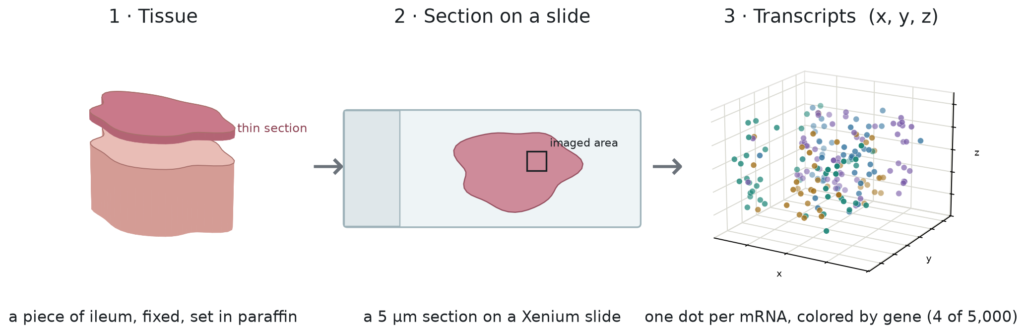
Each molecule becomes a dot with a gene name, a position (x, y, z), and a quality score. The panel also carries negative-control probes that match no real gene, so any dot they produce is a false detection. Counting those dots gives an estimate of how often false detections happen. We will use that estimate later in the series. Across the 16 sections, about 450 million dots ended up inside cells.
A Xenium run writes out a standard set of files. The team shared a processed version: one AnnData file (the standard Python format for single-cell
data) (.h5ad, about 9 GB) that holds the cell-level parts, plus their own annotations.
| Xenium output | What it holds | In this dataset? |
|---|---|---|
transcripts.parquet | every dot: gene, x, y, z, quality score, and the cell it was assigned to | No |
cell_boundaries.parquet, nucleus_boundaries.parquet | the outline drawn around each cell and nucleus | No |
| morphology images | the stain images used to find the cells | No |
cells.parquet | one row per cell: centroid, cell and nucleus area, dot and negative-control counts | Yes, as obs |
| cell-feature matrix | counts for each cell and gene | Yes, 2,131,098 cells × 5,001 genes |
| added by the authors | cell-type labels at several levels, spatial niches, embeddings | Yes |
So we have every cell and its gene counts, but not the individual dots or the outlines around the cells. Most of this note works from the cell table: where each cell sits, how big it is, and what type it is.
From dots to cells
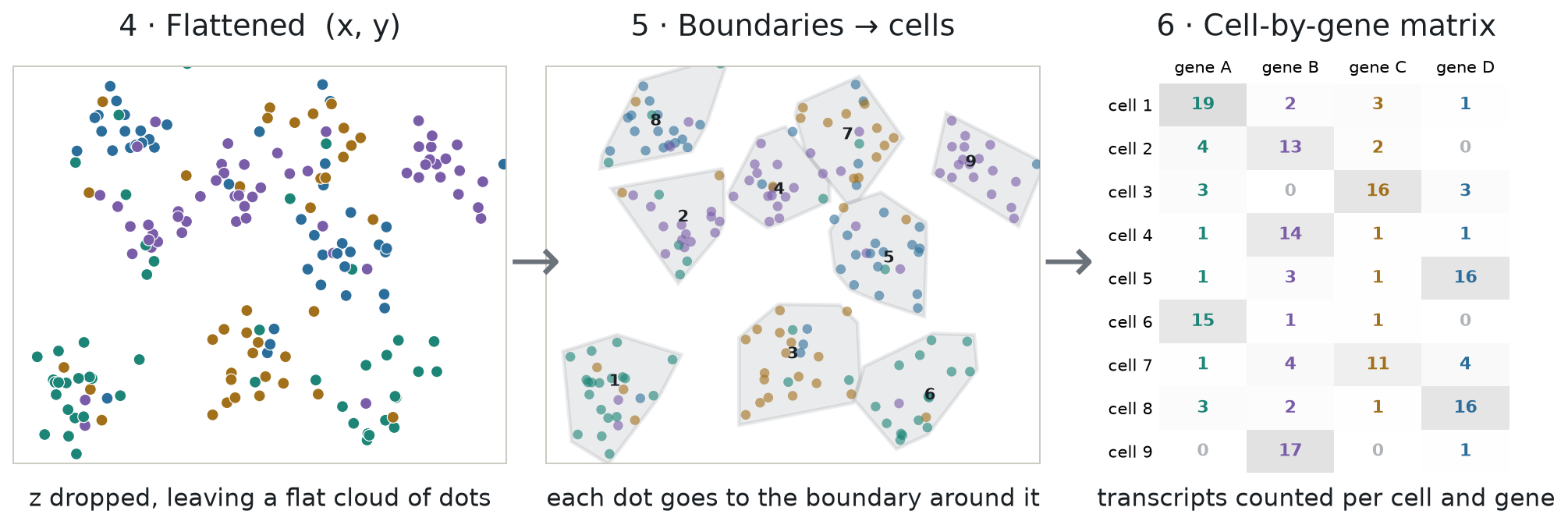
The cell table we have is the end product of a processing step: grouping the dots (the detected RNA molecules) into cells. The pipeline does this in three steps, panels 4 to 6 of Figure 2:
- Flatten the section: drop z, so the dots lie on a flat image. Because the section is about as thick as a small cell, flattening can stack two cells into one outline.
- Find the cells and draw an outline around each one.
- Assign each dot to the cell whose outline contains it.
Step 2 is called segmentation, and step 3 is called assignment. The standard rule for assignment is point-in-polygon. Counting the dots in each cell, gene by gene, gives the cell-by-gene matrix.
Figure 2. From dots to cells to a cell-by-gene matrix
In this study, the authors used Xenium's own segmentation, which traces each outline from the stain images in one of three ways, tried in order. It first looks for the cell's edge in a boundary stain that marks cell membranes (ATP1A1, CD45, and E-cadherin). Where that edge is unclear, it uses an interior stain (18S, which stains the RNA-rich inside of a cell). Where both fail, it takes the nucleus and grows it outward by 5 µm. The cell table records which of the three was used for every cell, so we can count them once the data is loaded.
Loading Xenium data in Python
The .h5ad file holds 2.1 million cells × 5,001 genes, about 9 GB on disk. For most of this note we only need the cell table (obs), so let's open the file with h5py and leave the expression matrix on
disk:
Show code: open the file
import h5py, pandas as pd

# show all columns of a wide table on one line
pd.set_option("display.width", 200, "display.max_columns", None)

# open the file; we read only the cell table (obs), the 9 GB matrix stays on disk
f = h5py.File("xenium5k_scVI_CellCharter_batch2_reannot_SCP.h5ad", "r")
obs = f["obs"]The file stores numbers as plain arrays and labels as codes plus a list of categories. This small helper reads either kind:
Show code: a helper that reads one column
def column(name):
    g = obs[name]
    # numbers are stored as plain arrays: read them as is
    if isinstance(g, h5py.Dataset):
        return g[:]
    # labels are stored as codes plus a list of categories: turn codes into names
return g["categories"].asstr()[:][g["codes"][:]]Now pick the columns we need, give them short names, and build a table:
Show code: build the cell table
# short names for the columns we need
cols = {"section": "biosample_id", "x": "x_centroid", "y": "y_centroid",
        "area": "cell_area", "dots": "transcript_counts",
        "cell_type": "megagut_lvl1_majority_voting", "outline": "segmentation_method"}

# build the table, one column at a time
cells = pd.DataFrame({short: column(name) for short, name in cols.items()})

# short names for the three ways an outline was drawn
outline_names = {"Segmented by boundary stain (ATP1A1+CD45+E-Cadherin)": "boundary stain",
                 "Segmented by interior stain (18S)": "interior stain",
                 "Segmented by nucleus expansion of 5.0µm": "nucleus expansion"}
cells["outline"] = cells.outline.map(outline_names)Let's look at it:
Show code: print the first rows
# number of cells (rows) and columns
print(cells.shape)

# the first three cells
print(cells.head(3).round(1))

# how many outlines came from each method
print(cells.outline.value_counts())(2131098, 7)
section x y area dots cell_type outline
0 0054175__GI10072_CD_adj 424.7 1034.2 49.1 236 Myeloid boundary stain
1 0054175__GI10072_CD_adj 542.6 872.8 68.0 555 T and NK cells boundary stain
2 0054175__GI10072_CD_adj 525.7 852.1 47.1 327 T and NK cells boundary stain
outline
interior stain 1705088
boundary stain 354259
nucleus expansion 71751
Name: count, dtype: int64Printing it gives:
Each row is one cell, with these columns:
| Column | Meaning |
|---|---|
section | which section the cell is in: a 7-digit donor ID, then a tag for the piece. Inflamed pieces are tagged inf, INF or affected; adjacent pieces adj, nor, NOR or adjacent. One ID, 0060032, covers two patients, told apart by specimen (gi9662, gi10056) |
x, y | the center of the cell's outline in µm, within its own section |
area | the area inside the outline, in µm² |
dots | how many dots (detected RNA molecules) fell inside the outline |
cell_type | the authors' label, one of seven broad lineages |
outline | how the outline was drawn (see above) |
For example, the first row is a myeloid cell from patient 0054175's adjacent piece, centered at
x = 424.7 µm and y = 1,034.2 µm. Its outline covers 49.1 µm², about the size of a circle 7.9 µm
across, and 236 dots fell inside it. Its outline came from the boundary stain. The x and y
values only make sense within one section, because every section has its own coordinates.
The counts at the bottom show how the outlines were made: 80% from the interior stain, 17% from the boundary stain, and 3% from growing the nucleus by 5 µm. So only about one cell in six has an outline drawn from the boundary stain, the stain that marks cell membranes.
The tissue, cell by cell
With the table loaded, a few lines of pandas tell us what the dataset holds. We start with the two kinds of piece. The section names carry the tag, so we can label each cell as inflamed or adjacent and count:
Show code: inflamed vs adjacent
from math import pi

# label each cell inflamed or adjacent, from the tag in its section name
cells["piece"] = (cells.section.str.lower().str.contains("inf|affected")
                  .map({True: "inflamed", False: "adjacent"}))

# sections and cells for each kind of piece
print(cells.groupby("piece").agg(sections=("section", "nunique"), cells=("section", "size")))

# the smallest, middle and largest section, in cells
print(cells.section.value_counts().agg(["min", "median", "max"]).astype(int)) sections cells
piece
adjacent 8 760733
inflamed 8 1370365
min 44286
median 112381
max 240888
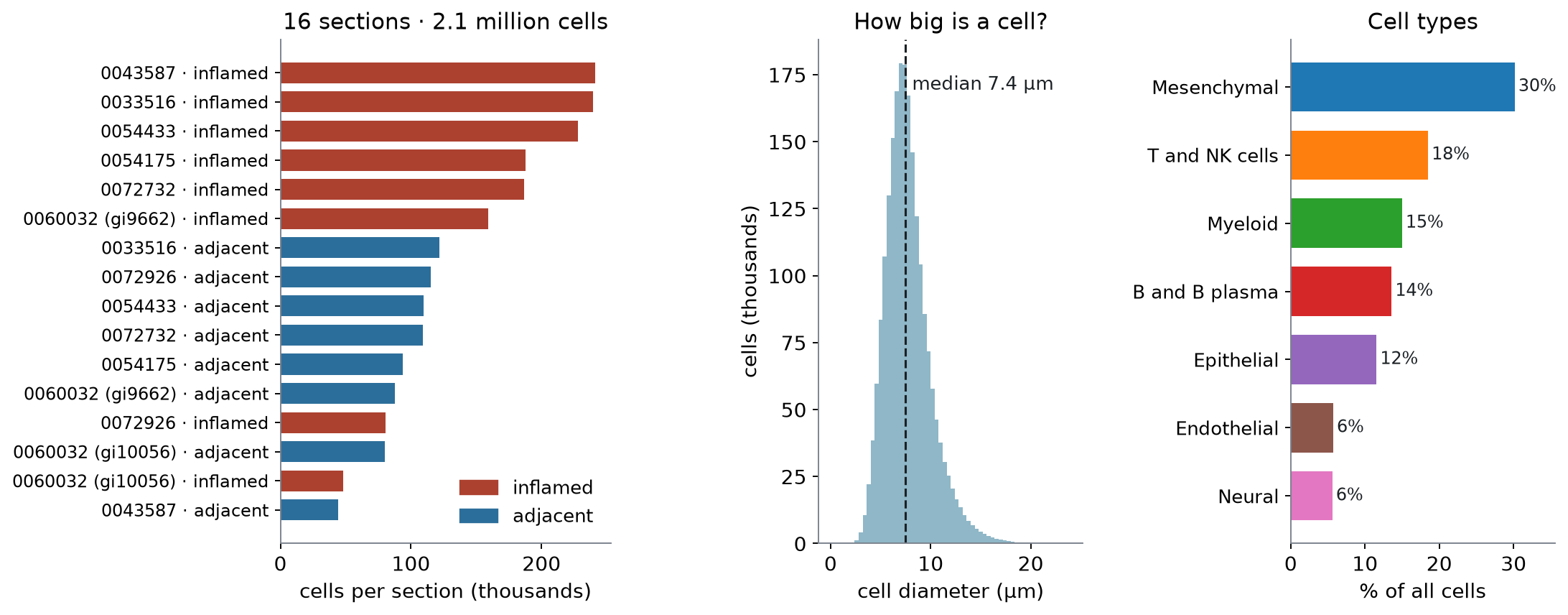
Name: count, dtype: int64There are eight inflamed pieces and eight adjacent ones, one of each per patient. The sections differ a lot in size, from about 44,000 to 241,000 cells, and the inflamed piece is the larger one for six of the eight patients. Next, the cell types:
Show code: cell-type shares
# share of all cells in each cell type
print(cells.cell_type.value_counts(normalize=True).round(2))cell_type
Mesenchymal 0.30
T and NK cells 0.18
Myeloid 0.15
B and B plasma 0.14
Epithelial 0.12
Endothelial 0.06
Neural 0.06
Name: proportion, dtype: float64Stromal (mesenchymal) and immune cells make up most of the tissue, and epithelial cells, the lining of the gut, are only 12%. Last, we look at cell size. The table gives each cell's area, so we convert it to the diameter of a circle with the same area:
Show code: cell size and dots
# diameter of a circle with the same area as the cell
diameter = 2 * (cells.area / pi) ** 0.5

# typical cell size and number of dots
print(f"median diameter {diameter.median():.1f} µm, median dots {cells.dots.median():.0f}")median diameter 7.4 µm, median dots 159A typical cell is about 7.4 µm across and holds 159 dots. Figure 3 shows the same three summaries:
Figure 3. The dataset at a glance: sections, cell size, and cell types
Zooming in, from sections to genes
Let's start with all 16 sections, pick one inflamed section, and zoom in until we reach single cells and the genes inside them. First we need a color for each cell type and two small helpers. One picks the cells inside a square, and the other tidies the axes:
Show code: setup for the maps
import re
import numpy as np
import matplotlib.pyplot as plt
from matplotlib.patches import Circle, Rectangle

# one color per cell type, most common type first
colors = dict(zip(cells.cell_type.value_counts().index, plt.get_cmap("tab10").colors))

def inside(df, x0, y0, w):
    # the cells whose centers fall inside a square (top-left corner x0, y0; width w; in µm)
    return df[(df.x >= x0) & (df.x < x0 + w) & (df.y >= y0) & (df.y < y0 + w)]

def tidy(ax, square=None):
    # same scale on both axes, and no tick labels
    ax.set_aspect("equal")
    ax.set_xticks([])
    ax.set_yticks([])
    # zoom to a square if one is given; y grows downward, as in the image
    if square:
        x0, y0, w = square
        ax.set_xlim(x0, x0 + w)
        ax.set_ylim(y0 + w, y0)
    else:
ax.invert_yaxis()Sixteen sections, an inflamed and an adjacent piece from each patient
Each section is drawn at the same scale, every cell a point colored by type. The framed one is the inflamed section we zoom into next:
Show code: draw all 16 sections
def label(section, piece):
    # patient ID, plus the specimen for the one patient with two (0060032)
    specimen = re.search(r"gi\d+", section)
    patient = section[:7] + (f" ({specimen.group()})" if section.startswith("0060032") else "")
    return f"{patient} · {piece}"

# order the sections by patient, inflamed first; draw them all at the same scale
sections = cells.groupby("section").piece.first().reset_index()
sections["label"] = [label(s, p) for s, p in zip(sections.section, sections.piece)]
sections["patient"] = sections.label.str.split(" · ").str[0]
sections = sections.sort_values(["patient", "piece"], ascending=[True, False])
span = cells.groupby("section")[["x", "y"]].agg(np.ptp).max().max()

fig, axes = plt.subplots(4, 4, figsize=(12, 12))
for ax, (_, row) in zip(axes.flat, sections.iterrows()):
    group = cells[cells.section == row.section]
    ax.scatter(group.x, group.y, s=0.05, c=group.cell_type.map(colors), linewidths=0)
    tidy(ax, (group.x.min(), group.y.min(), span))
    ax.set_title(row.label, fontsize=9)
    # frame the section we zoom into next
    if row.section == "0043587_affected":
        for spine in ax.spines.values():
            spine.set(color="black", linewidth=2.5)
plt.show()Figure 4. All 16 sections at the same scale; each point is a cell, colored by type
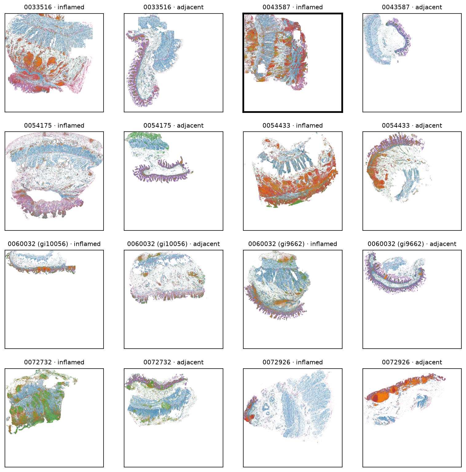
Each patient's two pieces sit side by side. They differ in size and shape, and in most of the inflamed pieces dense patches of immune cells are visible: red B and plasma cells, orange T cells, and in one patient (0072732) green myeloid cells.
One inflamed section: stroma, immune patches, and epithelium
We pick the framed section, the inflamed piece from patient 0043587, because it is the largest in the atlas, with 240,888 cells. It also holds more of the paper's inflammatory fibroblasts than any other section. Here it is on its own, large enough for the layout of the tissue to show. The box marks a 1 mm square near the top right, placed over an ulcer around the spot where those fibroblasts are most dense:
Show code: draw one section
# the inflamed section we zoom into, and a 1 mm square inside it (x0, y0, width in µm),
# placed around the patch below
one = cells[cells.section == "0043587_affected"]
region = (3679.39, 606.96, 1000)

def draw_section(ax):
    # most common type first, so rarer types are drawn on top and stay visible
    for cell_type, color in colors.items():
        group = one[one.cell_type == cell_type]
        ax.scatter(group.x, group.y, s=0.3, color=color, linewidths=0, label=cell_type)
    # mark the 1 mm square we zoom into next
    ax.add_patch(Rectangle(region[:2], region[2], region[2], fill=False))
    tidy(ax)

fig, ax = plt.subplots(figsize=(6, 6))
draw_section(ax)
handles = [plt.Line2D([], [], marker="o", ls="", color=c, label=t) for t, c in colors.items()]
ax.legend(handles=handles, fontsize=8, loc="upper left", bbox_to_anchor=(1.01, 1), frameon=False)
plt.show()Figure 5. The inflamed section from patient 0043587; each point is a cell
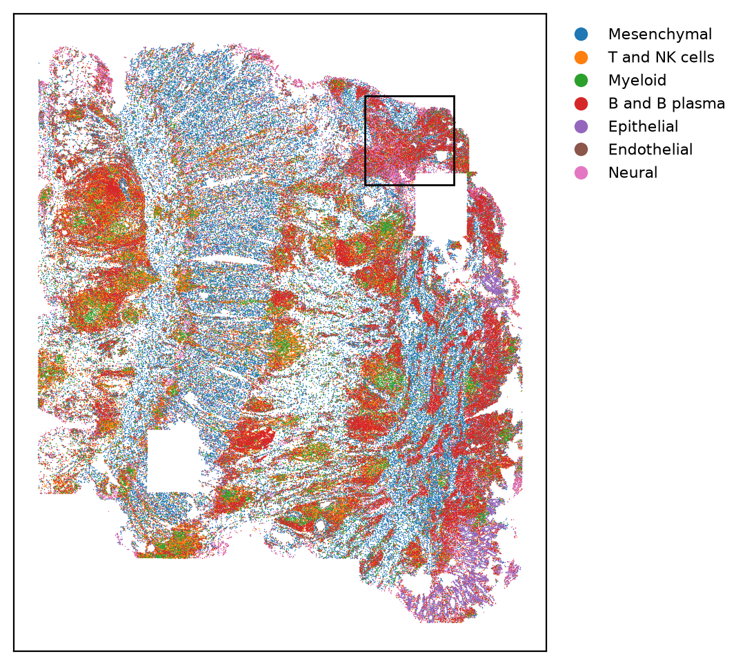
The cell types fall into clear regions: blue stroma, red patches of B and plasma cells, and the purple epithelial lining along the lower right. The two white rectangles are areas with no cells in the table.
A 1 mm square over an ulcer
The whole section is about 5.4 mm wide and 6.5 mm tall, so the 1 mm box covers a small part of it. The points are now big enough to tell apart, and instead of colored patches we can follow how the tissue is arranged: which cell types sit together, and where one kind of tissue ends and the next begins. The smaller box marks the 150 µm patch we zoom into after this:
Show code: draw the 1 mm square
# the 150 µm patch with the most inflammatory fibroblasts in the section (see choose_ulcer_patch.py)
patch = (4354.39, 756.96, 150)

def draw_region(ax):
    part = inside(one, *region)
    ax.scatter(part.x, part.y, s=3, c=part.cell_type.map(colors), linewidths=0)
    # mark the 150 µm patch we zoom into next
    ax.add_patch(Rectangle(patch[:2], patch[2], patch[2], fill=False))
    tidy(ax, region)

fig, ax = plt.subplots(figsize=(6, 6))
draw_region(ax)

# a color legend for the cell types
handles = [plt.Line2D([], [], marker="o", ls="", color=c, label=t) for t, c in colors.items()]
ax.legend(handles=handles, fontsize=8, loc="upper left", bbox_to_anchor=(1.01, 1), frameon=False)
plt.show()
# what the square holds: the cell types, and the share of cells in the ulcer niche (niche 11)
niche = pd.Series(column("spatial_cluster15"), index=cells.index)
square = inside(one, *region)
print(len(square), "cells")
print(square.cell_type.value_counts(normalize=True).round(2).to_string())
print(f"in the ulcer niche: {(niche[square.index] == '11').mean():.0%}")Figure 6. A 1 mm square over an ulcer; each point is a cell
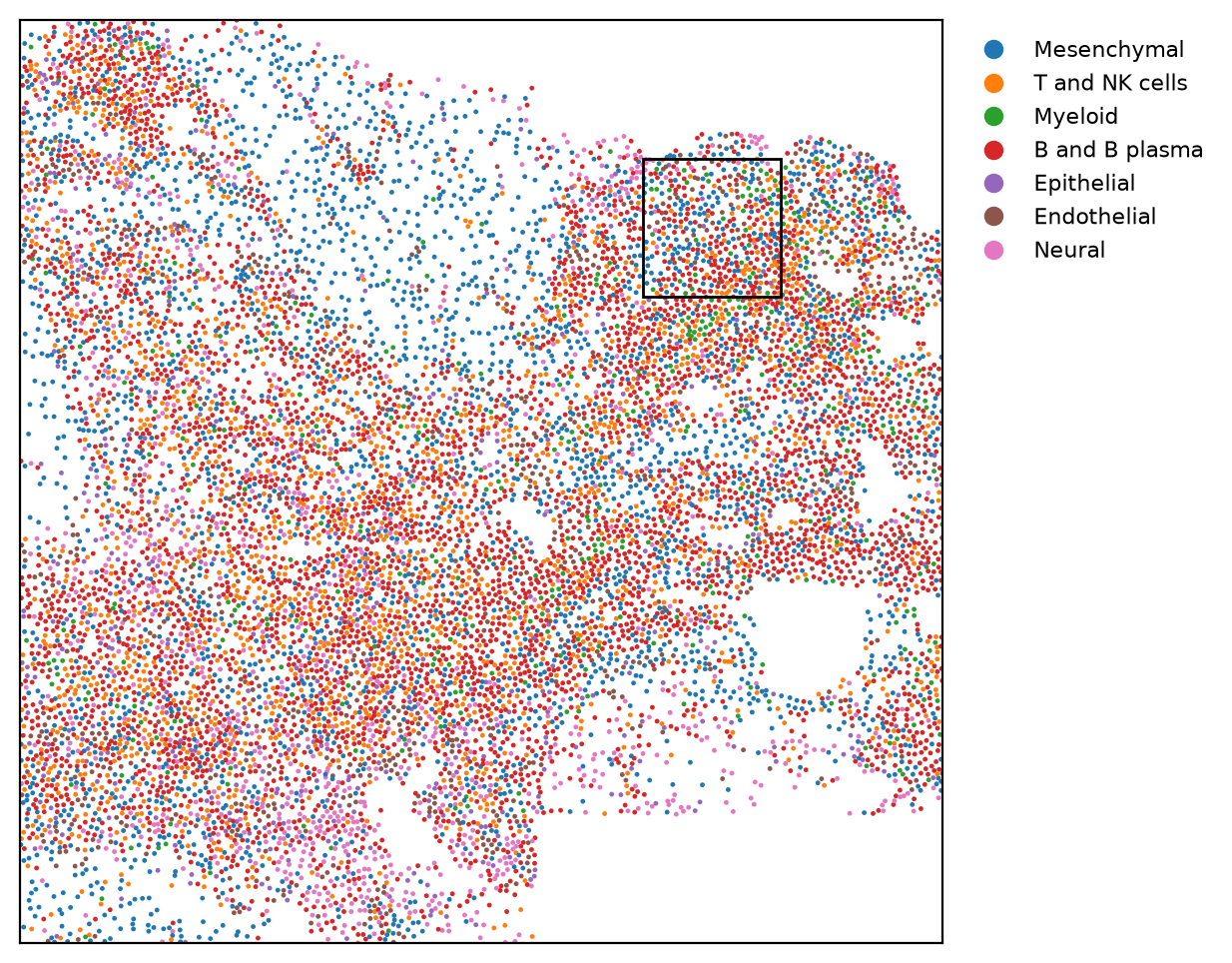
12367 cells
cell_type
B and B plasma    0.37
Mesenchymal       0.24
T and NK cells    0.15
Neural            0.09
Endothelial       0.08
Epithelial        0.04
Myeloid           0.04
in the ulcer niche: 70%This square holds 12,367 cells. B and plasma cells (37%) and stromal cells (24%) make up most of it, with T cells (15%) mixed in. The authors split the tissue into 15 neighborhoods of similar cells (they call them niches), and 70% of the cells in this square fall in the one they call the mucosal ulcer.
A 150 µm patch, with cells at their real size
At this scale we can draw each cell at its real size. The table gives each cell's center and area, but not the outline itself, because the outline files
(cell_boundaries.parquet) were not shared. So we draw each cell as a circle around its center,
with the same area as its real outline: radius = √(area / π). The size is right, but the shape is
a stand-in. Real cells are stretched and irregular, and two real outlines never cross, while two
circles can:
Show code: draw the patch
patch_cells = inside(one, *patch)

def draw_patch(ax, color_of):
    for _, cell in patch_cells.iterrows():
        # a circle at the cell's center, with the same area as its outline
        radius = (cell.area / np.pi) ** 0.5
        ax.add_patch(Circle((cell.x, cell.y), radius, color=color_of(cell), alpha=0.8))
    tidy(ax, patch)

fig, ax = plt.subplots(figsize=(6, 6))
draw_patch(ax, lambda cell: colors[cell.cell_type])

# a color legend for the cell types
handles = [plt.Line2D([], [], marker="o", ls="", color=c, label=t) for t, c in colors.items()]
ax.legend(handles=handles, fontsize=8, loc="upper left", bbox_to_anchor=(1.01, 1), frameon=False)
plt.show()
# what the patch holds: the cell types, and the share of cells in the ulcer niche
print(len(patch_cells), "cells")
print(patch_cells.cell_type.value_counts().to_string())
print(f"in the ulcer niche: {(niche[patch_cells.index] == '11').mean():.0%}")Figure 7. A 150 µm patch; each circle is a cell, drawn at its own area
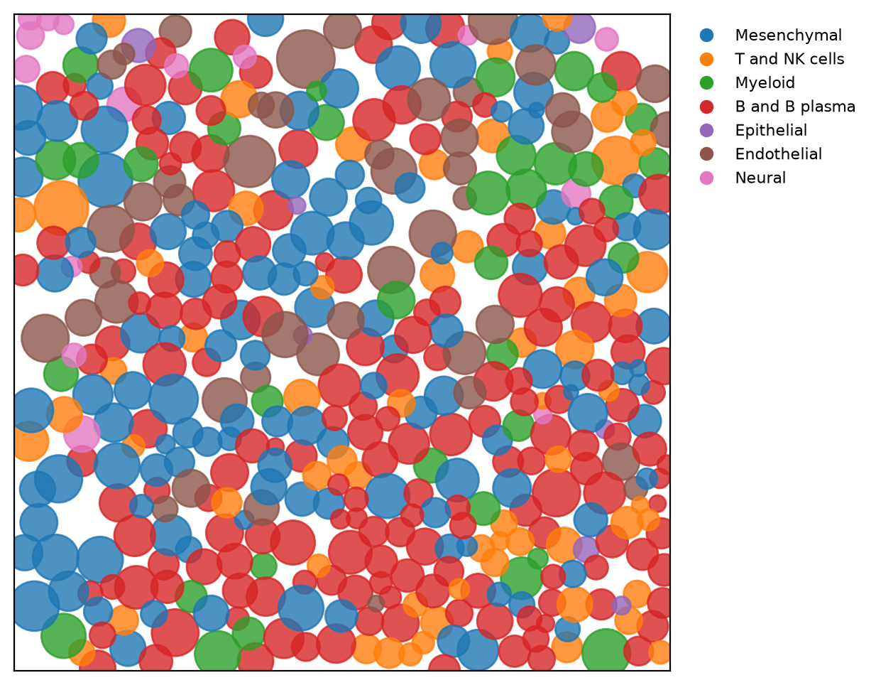
459 cells
cell_type
B and B plasma    171
Mesenchymal       123
T and NK cells     62
Endothelial        45
Myeloid            36
Neural             15
Epithelial          7
in the ulcer niche: 88%The patch holds 459 cells, and 88% of them are in the ulcer neighborhood. They are B and plasma cells (red), stromal cells (blue), T cells (orange), blood-vessel cells (brown), and myeloid cells (green). The cells sit packed against each other. Where two circles overlap, that is a limit of the circles: real outlines meet but do not cross.
The three zooms side by side
With the drawing functions defined, putting the three zooms side by side takes a few lines:
Show code: the three zooms side by side
fig, axes = plt.subplots(1, 3, figsize=(15, 5.5))
draw_section(axes[0])
draw_region(axes[1])
draw_patch(axes[2], lambda cell: colors[cell.cell_type])
plt.show()Here is a polished version of that figure, with scale bars and lines that link each square to the next. The script that draws it is in the repo:
Figure 8. One section at three scales
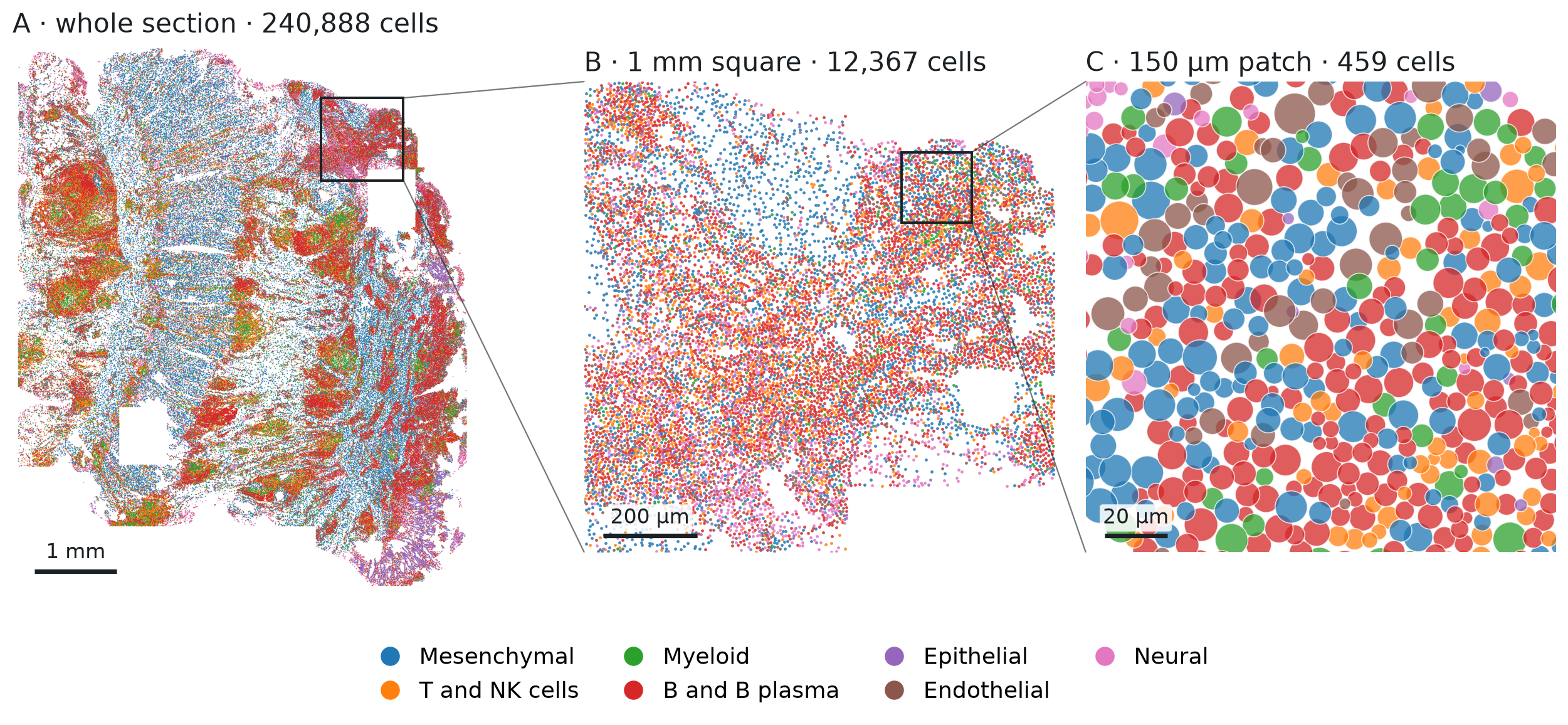
Inflammatory fibroblasts in the ulcer, and their marker gene
The paper focuses on inflammatory fibroblasts, a fibroblast state the authors found mainly in
ulcers like this one. The authors'
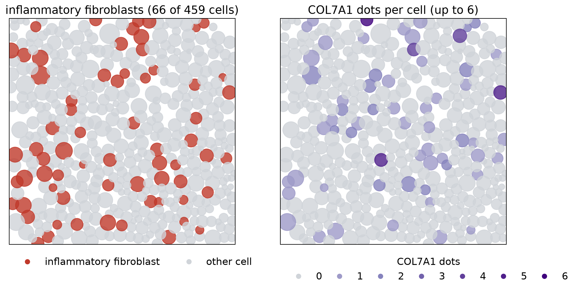
finer labels (annot_new) call it "COL7A1hi inflammatory fibroblast", after a gene it expresses more highly than other fibroblasts do. The individual dots were not shared, so we cannot see where a gene's dots are inside a cell. We do
have a count for every gene in every cell: how many dots of that gene fell inside the cell's outline. The authors made the label from the same expression data, so the counts should agree with it. The
code below shows that agreement cell by cell. It marks the inflammatory fibroblasts in the patch, then
shades every cell by its COL7A1 count, read from the sparse count matrix on disk (a matrix that
stores only the nonzero counts):
Show code: read gene counts, shade the patch, and measure expression
# the authors' finer labels, for the cells in the patch
fine = pd.Series(column("annot_new")[patch_cells.index], index=patch_cells.index)
is_if = fine == "M COL7A1hi inflammatory fibroblast"

# the raw counts: a sparse matrix on disk, one row per cell, one column per gene
counts = f["layers"]["counts"]
genes = list(f["var"]["_index"].asstr()[:])

def gene_counts(rows, name):
    # read only the rows we need; each row stores its nonzero genes (indices) and counts (data)
    g = genes.index(name)
    out = []
    for r in rows:
        start, end = counts["indptr"][r], counts["indptr"][r + 1]
        idx, val = counts["indices"][start:end], counts["data"][start:end]
        out.append(val[idx == g].sum())
    return pd.Series(out, index=rows)

col7a1 = gene_counts(patch_cells.index, "COL7A1")

fig, axes = plt.subplots(1, 2, figsize=(12, 6))

# left: inflammatory fibroblasts in red, every other cell in gray
draw_patch(axes[0], lambda cell: "#c0392b" if is_if[cell.name] else "#d0d4d9")
axes[0].set_title(f"inflammatory fibroblasts ({is_if.sum()} of {len(is_if)} cells)", fontsize=15)

# right: COL7A1 dots per cell; gray = none, light to dark purple = 1 up to the most in the patch
top = col7a1.max()
def shade(cell):
    n = col7a1[cell.name]
    return "#d0d4d9" if n == 0 else plt.cm.Purples(0.4 + 0.6 * n / top)
draw_patch(axes[1], shade)
axes[1].set_title(f"COL7A1 dots per cell (up to {top:.0f})", fontsize=15)

# keys: red vs gray on the left, the number of COL7A1 dots on the right
def key(color, label):
    return plt.Line2D([], [], marker="o", ls="", color=color, label=label)

left = [key("#c0392b", "inflammatory fibroblast"), key("#d0d4d9", "other cell")]
axes[0].legend(handles=left, loc="upper left", bbox_to_anchor=(0, -0.02), ncol=2, frameon=False,
               fontsize=13)
right = [key("#d0d4d9", "0")]
right += [key(plt.cm.Purples(0.4 + 0.6 * n / top), str(n)) for n in range(1, int(top) + 1)]
axes[1].legend(handles=right, title="COL7A1 dots", loc="upper left", bbox_to_anchor=(0, -0.02),
               ncol=len(right), frameon=False, fontsize=13, title_fontsize=13, columnspacing=0.8)
plt.show()

# how many cells hold 0, 1, 2, ... COL7A1 dots, for inflammatory fibroblasts and for other cells
group = is_if.map({True: "inflammatory fibroblast", False: "other cell"})
table = pd.crosstab(group, col7a1.astype(int), rownames=[""], colnames=["COL7A1 dots"])
print(table.reindex(columns=range(int(top) + 1), fill_value=0))

# expression: COL7A1 dots per 1,000 dots in the cell, which corrects for how many dots the cell holds
per_1000 = 1000 * col7a1 / patch_cells.dots
print(pd.DataFrame({"total dots (median)": patch_cells.dots.groupby(group).median(),
                    "COL7A1 per 1,000 dots (mean)": per_1000.groupby(group).mean().round(1)}))

# the broad labels of the inflammatory fibroblasts
print(patch_cells.cell_type[is_if].value_counts().to_string())Figure 9. Inflammatory fibroblasts and their marker gene, COL7A1, in the patch
COL7A1 dots                0   1   2  3  4  5  6

inflammatory fibroblast   30  22  10  0  1  2  1
other cell               368  19   5  0  1  0  0
                         total dots (median)  COL7A1 per 1,000 dots (mean)
inflammatory fibroblast                271.0                           3.4
other cell                             144.0                           0.4
cell_type
Mesenchymal       56
B and B plasma     7
T and NK cells     2
Epithelial 1Of the 459 cells, 66 are inflammatory fibroblasts (left), and the COL7A1 dots (right) fall mostly on the same cells. The table and the summary below it compare the two groups:
- Cells with at least one COL7A1 dot: 36 of the 66 inflammatory fibroblasts (55%), against 25 of the other 393 cells (6%).
- Total dots: inflammatory fibroblasts hold more dots, a median of 271 against 144, so raw COL7A1 counts would overstate the difference.
- Expression, as COL7A1 dots per 1,000 dots in the cell: 3.4 against 0.4, about eight times more in the inflammatory fibroblasts.
The match is still loose. The counts are small, at most 6 dots in a cell, so a cell can make the gene and still show none. The labels are not perfect either: in the broad labels, 56 of the 66 are stromal cells, 7 are called B or plasma cells, and 3 are other types.
Across the atlas, these cells are found almost only in the inflamed pieces. Counting them in every section shows where:
Show code: count inflammatory fibroblasts in every section
# inflammatory fibroblasts in every section, from most to fewest
fine_all = pd.Series(column("annot_new"), index=cells.index)
is_if_all = fine_all == "M COL7A1hi inflammatory fibroblast"
per_section = is_if_all.groupby([cells.piece, cells.section]).sum().sort_values(ascending=False)
print(per_section.to_string())
print(f"share in inflamed pieces: {is_if_all[cells.piece == 'inflamed'].sum() / is_if_all.sum():.0%}")piece section
inflamed 0043587_affected 2328
0054433__GI9676_CD_inf 1871
0033516_affected 1111
0072732__CD10500INF 784
adjacent 0054433__GI9676_CD_adj 114
inflamed 0054175__GI_10072_CD_inf 36
adjacent 0072732__CD10500NOR 21
0060032__gi10056_nor 20
0033516_adjacent 14
inflamed 0060032__gi9662_inf 9
adjacent 0072926__CD9623NOR 7
0054175__GI10072_CD_adj 3
0043587_adjacent 2
inflamed 0060032__gi10056_inf 2
0072926__CD9623INF 2
adjacent 0060032__gi9662_nor 1
share in inflamed pieces: 97%Of the 6,325 in the atlas, 97% are in inflamed pieces, and most of those are in just four of the eight: those four hold 784 to 2,328 each, while the other four inflamed pieces hold 36 or fewer. Seven of the eight adjacent pieces hold 21 or fewer.
Summary and what comes next
What we saw in this first look:
- The data. 2.1 million cells from 16 sections of ileum, an inflamed and an adjacent piece from each of eight patients. The shared file holds the cell table and the gene counts. The dots and the cell outlines were not shared.
- The outlines. Each cell's outline was drawn once, by Xenium. 80% came from the interior stain, and only about one in six was drawn from the boundary stain.
- The tissue. Stromal and immune cells make up most of it, and a typical cell is about 7.4 µm across with 159 dots.
- The zoom. In one inflamed section, an ulcer packed with immune cells holds the paper's inflammatory fibroblasts, and in our patch they express about eight times more COL7A1 than the other cells. These fibroblasts are almost absent from the adjacent pieces.
Each cell's outline is drawn once, and every dot inside it is counted for that cell. Yet the cells in Figure 7 are packed close together, the 5 µm section can hold parts of two cells stacked on top of each other, and a cell holds only a few dots of any one gene. If some of the dots near an outline belong to the neighboring cell, how many cells' counts change, and by how much?
The next note takes that up with the same table: how closely neighboring cells are packed, how often neighbors are a different cell type, and what that could do to the counts. A companion note asks the other question this atlas raises: which cell types change in inflammation, using the inflamed and adjacent pieces from all eight patients.
Reproduce
Data. One AnnData file, xenium5k_scVI_CellCharter_batch2_reannot_SCP.h5ad (about 9 GB), from
the study's page on the
Broad Single Cell Portal. The
download is free but needs a Google sign-in.
Environment. Python 3.9 or later, with h5py, pandas, numpy, and matplotlib.
Code. Start Python in the folder that holds the file (the notebook in the repo expects it in data/),
and run the code blocks above in order, in
one session; each block uses names defined by the blocks before it. Reading the cell table takes a
few seconds, and the 16-section map about ten seconds. All of it, as a notebook and as the scripts
behind the finished figures, is in
tensoromics/notes/spatial-xenium-crohns:
| Figures | Where |
|---|---|
| 1, 2 | scripts/pipeline_fig.py (drawn from made-up dots, no data needed) |
| 3 | scripts/crohn_summary.py |
| 4–7, 9 | the code blocks above, also in spatial-transcriptomics-crohns-xenium.ipynb |
| 8 | scripts/crohn_zoom.py (reads a cell table saved first by scripts/extract_crohn_obs.py) |
scripts/choose_ulcer_patch.py shows how the 1 mm square and the 150 µm patch were chosen.
Working on something like this?
I take on consulting work in this area. See Multi-Omics Data Analysis or get in touch.